

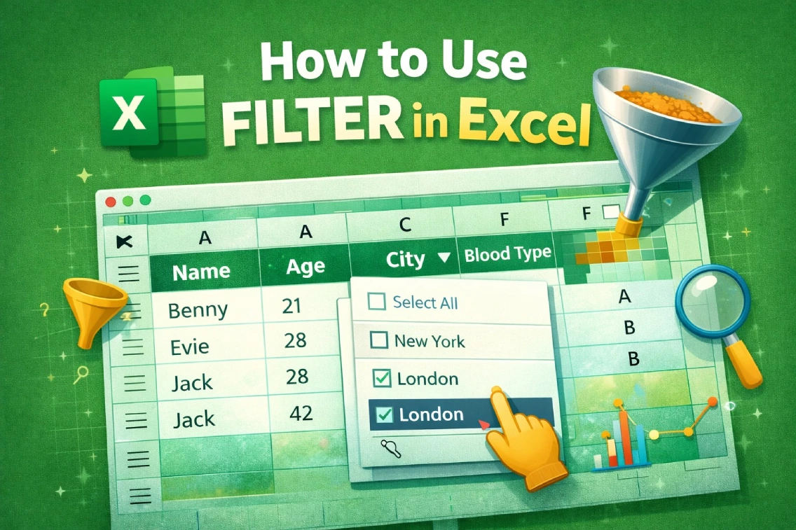
Introduction
Excel is a very useful tool for students to organise, study, and understand information easily. When working with long lists or tables, finding specific details can be confusing. This is where filtering in Excel helps. In this article, I’ll explain what filtering means, how to use it, different types of filters, examples, common mistakes, and quick FAQs.
What Does “Filter” Mean in Excel?
In Excel, a filter means hiding the data you do not need and showing only the information that is important at that moment. For example, you can filter marks to see only scores above 80, filter names by class, or filter items by category. The best part is that filtering does not delete any data. All the information is still there; Excel only hides the unwanted rows temporarily until you remove the filter.
Why Filtering Is Useful for Students
Filtering is very helpful for students because it makes large data easy to manage. It helps you find answers quickly without scrolling again and again. You can compare values, analyse marks, and study patterns easily. Filters are useful for school projects, surveys, science experiments, attendance sheets, and exam results. They save time and reduce mistakes while working with data.
How to Apply a Basic Filter in Excel
If you are wondering how to make filter in Excel, follow these simple steps:
Step 1: Select the entire table or click on any one cell inside your data.
Step 2: Go to the Data tab on the ribbon at the top.
Step 3: Click on Filter (the small funnel icon).
Step 4: Small arrows will appear next to each column heading.
Step 5: Click the arrow in the column you want to filter.
Step 6: Choose the value or condition you need.
Example:
If you have a list of students with marks, click the arrow in the Marks column and choose Number Filters → Greater Than → 75. Excel will now show only students who scored above 75.
Types of Filters in Excel
Excel offers different types of filters based on the kind of data you are using.
Text Filters
Text filters are used for names, subjects, or categories.
Examples include begins with, ends with, contains, and does not contain.
For instance, you can filter names that begin with “A”.
Number Filters
Number filters are useful for marks, prices, or quantities.
Options include greater than, less than, between, and Top 10.
Example: show marks between 60 and 90.
Date Filters
Date filters help with attendance sheets and project timelines.
You can filter by today, this month, before, or after a date.
Custom Filters
Custom filters allow two conditions together.
Example: marks greater than 70 and less than 90.
How to Clear or Remove a Filter
After filtering, you may want to see all your data again.
To remove a single filter, click the filter arrow and select Clear Filter From…
To remove all filters at once, go to the Data tab and click Clear.
You can also use the remove filter in Excel shortcut by pressing Ctrl + Shift + L.
Clearing filters brings back the full data and does not change or delete anything.
Solved Examples
Example 1: Filter by Marks
A student list shows names and marks. Use Number Filters → Greater Than → 80 to see top scorers.
Example 2: Filter by Category
In a book list, click the Category column and select Science to show only science books.
Example 3: Filter by Date
In an attendance sheet, use Date Filters → Last 7 Days to view recent entries only.
Each example uses a different filter type for clarity.
Common Mistakes Students Make
Many students forget to include column headings before applying filters. Some apply filters to only part of the table, which causes errors. Others forget that rows are hidden and think data is missing. A common mistake is editing data while filters are still on.
Correct note:
Always select the full table, check for hidden rows, and clear filters before making changes.
Practice Exercises
Try these exercises on your own:
- Filter a list of numbers to show values greater than 50.
- Filter a class list to display only students in Grade 8.
- Filter a date column to show entries from January only.
Practising all filter types will make Excel much easier.
FAQs
What is the easiest way to apply a filter in Excel?
Select your data and press Ctrl + Shift + L (apply filter shortcut).
Can I filter more than one column at the same time?
Yes, Excel allows multiple column filters together.
Why can’t I see some data after filtering?
The rows are hidden due to active filters. Clear them to see all data.