

If you’ve ever worked on a large Excel sheet, you know the struggle. You scroll to the right to check some data, and suddenly the names, IDs, or categories on the left vanish. Now you’re guessing which row belongs to what—and that’s how mistakes happen.
Freezing columns in Excel solves this problem neatly. It lets you keep important columns visible while you scroll through the rest of the sheet. In this guide, I’ll show you how to freeze multiple columns in Excel, when it makes sense to use this feature, and a few common mistakes to watch out for.
What Does Freezing Columns Mean in Excel?
Freezing columns in Excel simply means locking certain columns in place so they stay visible when you scroll horizontally. The data doesn’t change—only how it appears on your screen.
This is different from hiding columns. When you hide a column, it disappears completely. Freezing keeps the column visible at all times, which is far more useful when you need constant reference.
You’ll often see frozen columns used in:
- Student records and attendance sheets
- Sales and finance reports
- Large tracking or comparison sheets
Basically, anytime the first few columns matter, freezing is a smart move.
When Should You Freeze Multiple Columns in Excel?
Freezing multiple columns is especially helpful when:
- You’re working with wide spreadsheets that stretch across many columns
- Important reference details like names, roll numbers, or product IDs need to stay visible
- You’re comparing data across several columns
- You’re doing data entry or verification and want to avoid mix-ups
If you’re constantly scrolling left just to remind yourself what a row refers to, it’s time to freeze those columns.
How to Freeze Multiple Columns in Excel (Step-by-Step)
Step 1 – Select the Right Column
This is the part most people get wrong the first time.
Excel freezes everything to the left of the column you select.
Example:
If you want to freeze Column A and Column B, click on Column C.
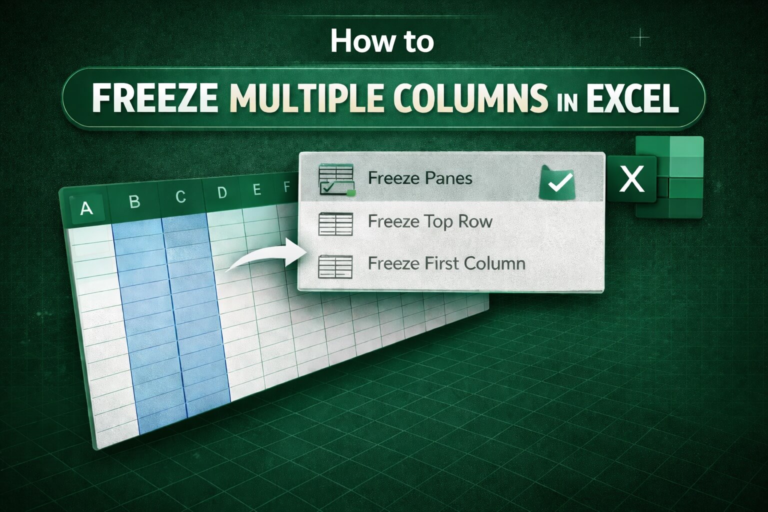
Step 2 – Open the Freeze Panes Option
- Go to the View tab at the top
- Click on Freeze Panes
Step 3 – Click Freeze Panes
- Select Freeze Panes from the dropdown
- Excel will immediately freeze the selected columns
You’ll see a thin grey line showing where the freeze starts.
How to Freeze Both Rows and Multiple Columns Together
Sometimes you want the best of both worlds—frozen headers at the top and frozen columns on the side.
Here’s how:
- Click the cell that is below the rows and to the right of the columns you want to freeze
- Go to View → Freeze Panes → Freeze Panes
This works beautifully for large reports where headings and key reference columns need to stay visible at all times.
How to Unfreeze Columns in Excel
If you want to remove the freeze:
- Go to the View tab
- Click Freeze Panes
- Choose Unfreeze Panes
Your sheet will return to normal scrolling instantly.
Common Mistakes to Avoid
- Selecting the wrong column before clicking Freeze Panes
- Trying to freeze columns after scrolling far across the sheet
- Mixing up Freeze Panes with the Split option
- Forgetting to unfreeze columns before sharing the file with others
These are small mistakes, but they can cause a lot of confusion.
Pro Tips for Smoother Excel Work
- Freeze only the most important columns—too many can feel cluttered
- Combine frozen rows and columns for large datasets
- Use freezing in dashboards, trackers, and monthly reports
Once you get used to it, freezing becomes second nature.
Conclusion
Freezing multiple columns in Excel is a simple feature, but it makes a huge difference when working with large spreadsheets. It keeps important information visible, reduces scrolling back and forth, and helps prevent errors. Whether you’re handling student data, financial reports, or tracking sheets, freezing columns can save time and make your work much easier. Best of all, it’s quick to set up and just as easy to remove.
FAQs
How many columns can I freeze in Excel?
You can freeze as many adjacent columns as you want.
Can I freeze columns and rows at the same time?
Yes, just select the correct cell and use Freeze Panes.
Why is the Freeze Panes option greyed out?
This usually happens if you’re editing a cell or working in a protected sheet.
How do I freeze the first two columns quickly?
Select Column C, then go to View → Freeze Panes → Freeze Panes.
What’s the difference between Freeze Panes and Split?
Freeze Panes locks parts of the sheet, while Split only divides the screen for viewing.
Does freezing affect formulas or data?
No. It only changes how the sheet looks on your screen.