

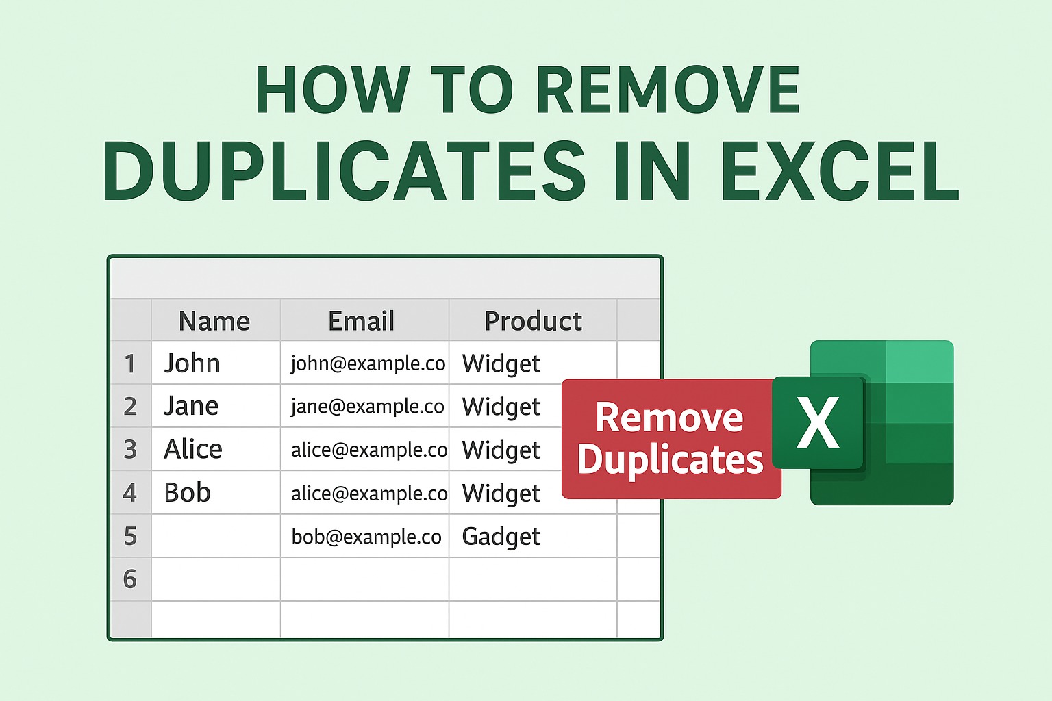
If you’ve ever opened an Excel sheet and felt overwhelmed because the same name or email appears again and again, trust me — you’re not alone. It happens to all of us. Maybe someone copied a list twice, maybe you pasted something in a hurry, or maybe the file has been passed around too many times. Either way, duplicates can make your data messy, confusing, and honestly a bit annoying.
The good news? Getting rid of them is much easier than people think. Excel actually has a built-in tool that cleans duplicates in seconds — and once you know where it is, you’ll wonder why you didn’t use it earlier.
Let me walk you through it in the simplest way possible.
What are duplicates, really?
Duplicates are just repeated entries.
That’s it. Nothing fancy.
For example:
- The same phone number typed twice
- Two rows with identical details
- An email ID that somehow appears five times
Left as it is, this can mess with your reports and throw off totals. Cleaning them keeps your data neat and dependable.
First step: Select the data
Before Excel can help you, it needs to know what to check.
You can:
- Highlight a single column
- Select multiple columns
- Or simply press Ctrl + A if you want it to look at everything
If you’re not sure where the duplicates are, Ctrl + A is the safest bet.
Next: Use Excel’s Remove Duplicates button
This is where the magic happens.
Go to the Data tab on top, and you’ll see a button called Remove Duplicates.
Click it.
No formulas, no complicated steps — just one button.
Now tell Excel what to compare
A small box pops up, showing your column names. This is Excel asking:
“Okay, what should I check for duplicates?”
If you only care about unique email IDs, select just the Email column.
If you want entire rows checked (meaning all values must match), select all columns.
Quick tip:
Tick the My data has headers option so Excel doesn’t treat your headings as actual data.
Time for the results
Hit OK and Excel will instantly scan your selection and clean things up.
You’ll get a message like:
“10 duplicate values found and removed; 90 unique values remain.”
It’s short, clear, and honestly feels a bit satisfying.
If you want to keep your original list untouched
Sometimes you don’t want Excel to delete anything — you just want a clean copy.
For that, there’s the Advanced Filter:
- Go to Data → Advanced
- Choose Copy to another location
- Tick Unique records only
- Select where you want the clean list to appear
Excel will place only the unique values in a new spot, leaving your original data safe.
If you prefer formulas
Some people enjoy formulas more than buttons. If that’s you, here are two useful ones:
For Excel 365 & 2021
=UNIQUE(range)
This immediately gives you a list of unique values.
For older Excel
=IF(COUNTIF($A$1:A1, A1)=1, A1, “”)
This one helps you spot duplicates by checking how many times a value has already appeared.
A quick keyboard shortcut
There isn’t a single key for removing duplicates, but this is the fastest keyboard method:
Alt → A → M
Literally just press those keys one after another:
- Alt opens the ribbon
- A goes to the Data tab
- M opens Remove Duplicates
Super quick once you get used to it.
A few things I always keep in mind
- I always take a backup before removing duplicates — just in case.
- Sometimes duplicates don’t look like duplicates because of extra spaces.
- Conditional Formatting (Home → Duplicate Values) is a great way to see duplicates before deleting them.
- If I’m unsure, I use the Advanced Filter method so nothing gets deleted accidentally.