by Bethany Institutions | Feb 16, 2026
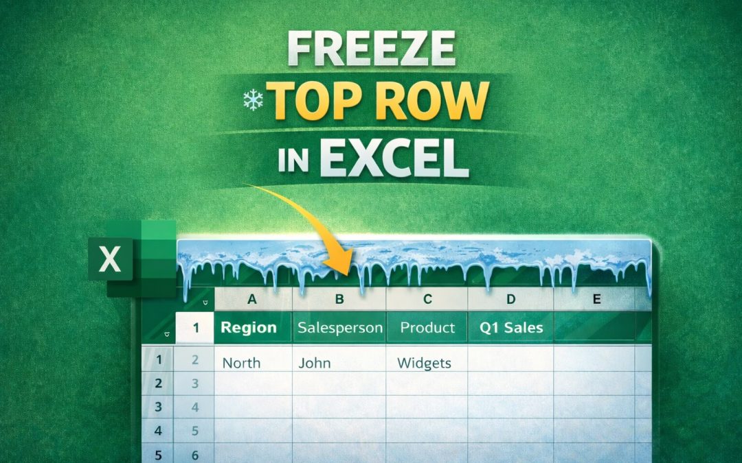
Freezing the top row in Excel helps you keep column headings visible while scrolling through large data sets.
When you work with long Excel sheets, it’s easy to forget what each column represents once you scroll down. Freezing the top row solves this problem by keeping your headers fixed at the top while the rest of the data moves. This feature is especially useful for school records, attendance sheets, marks lists, and office reports.
What Does “Freeze Top Row” Mean in Excel?
Freezing the top row in Excel means locking the first row of your worksheet so it remains visible even when you scroll down.
What stays visible
- The first row (usually column headings)
- Labels such as Name, Roll Number, Marks, Date, etc.
What moves while scrolling
- All rows below the frozen row
- Large sets of data without losing context
Why Should You Freeze the Top Row?
Freezing rows may seem like a small feature, but it makes a big difference when handling data.
Keeps headings visible
You always know what each column stands for, even in long sheets.
Reduces errors
No confusion while entering or checking data, especially in student marks or financial sheets.
Improves readability
Makes Excel sheets easier to read, understand, and present.
When to Use Freeze Top Row
You should use the freeze top row option whenever your Excel sheet has more data than what fits on one screen.
Long datasets
Sales data, survey responses, or monthly reports.
Tables with headers
Any sheet where the first row contains column names.
Student marks / attendance sheets
Teachers and school administrators find this feature extremely useful for daily work.
How to Freeze the Top Row in Excel
Freezing the top row in Excel is quick and easy.
Steps
- Open your Excel worksheet
- Click on the View tab in the top menu
- Select Freeze Panes
- Click on Freeze Top Row
That’s it! Your first row is now fixed.
This method works for:
- How to freeze top row in Excel
- How to lock a row in Excel
- How to fix the first row in Excel
- Cell freeze in Excel
How to Freeze 2 Rows in Excel (or More)
If you want to freeze cells in Excel beyond one row, follow these steps:
- Select the row below the rows you want to freeze
(For freezing 2 rows, click on Row 3) - Go to the View tab
- Click Freeze Panes
- Select Freeze Panes (not Freeze Top Row)
This is useful when you have multiple header rows.
How to Freeze First Two Columns in Excel
To freeze columns instead of rows:
- Select the column after the columns you want to freeze
(For two columns, click Column C) - Go to View
- Click Freeze Panes
- Select Freeze Panes
This answers the common query: how to freeze the first two columns in Excel.
How to Unfreeze the Top Row
If you no longer need the frozen row, you can easily remove it.
Steps
- Go to the View tab
- Click Freeze Panes
- Select Unfreeze Panes
This will:
- Unfreeze the top row
- Unfreeze columns
- Unfreeze the entire Excel sheet
This works for:
- How to unfreeze columns in Excel
- How to unfreeze Excel sheet
Freeze Top Row vs Freeze First Column
| Feature | Freeze Top Row | Freeze First Column |
| Purpose | Keeps headers visible | Keeps key identifiers visible |
| Use cases | Tables, marks sheets | Names, IDs, roll numbers |
| Scrolling | Vertical | Horizontal |
You can also freeze both rows and columns together using Freeze Panes.
Common Mistakes While Freezing Rows
Wrong row selected
Selecting the wrong cell before clicking Freeze Panes may freeze unwanted rows.
Using Freeze Panes incorrectly
Remember:
- Freeze Top Row = only first row
- Freeze Panes = multiple rows or columns
Confusing freeze with split
Split divides the screen into sections, while freeze locks rows or columns in place.
FAQs
Can I freeze more than one row?
Yes. Select the row below the rows you want to freeze and use Freeze Panes.
Why is Freeze Top Row not working?
Make sure:
- You are not in Page Layout view
- Your worksheet is not protected
- No cells are merged in the top row
Does freezing affect printing?
No. Freezing rows does not change how your sheet is printed.
Can I use this in Excel Online?
Yes, but options may be limited compared to the desktop version.
by Bethany Institutions | Jan 7, 2026
Introduction
Excel is a very useful tool for students to organise, study, and understand information easily. When working with long lists or tables, finding specific details can be confusing. This is where filtering in Excel helps. In this article, I’ll explain what filtering means, how to use it, different types of filters, examples, common mistakes, and quick FAQs.
What Does “Filter” Mean in Excel?
In Excel, a filter means hiding the data you do not need and showing only the information that is important at that moment. For example, you can filter marks to see only scores above 80, filter names by class, or filter items by category. The best part is that filtering does not delete any data. All the information is still there; Excel only hides the unwanted rows temporarily until you remove the filter.
Why Filtering Is Useful for Students
Filtering is very helpful for students because it makes large data easy to manage. It helps you find answers quickly without scrolling again and again. You can compare values, analyse marks, and study patterns easily. Filters are useful for school projects, surveys, science experiments, attendance sheets, and exam results. They save time and reduce mistakes while working with data.
How to Apply a Basic Filter in Excel
If you are wondering how to make filter in Excel, follow these simple steps:
Step 1: Select the entire table or click on any one cell inside your data.
Step 2: Go to the Data tab on the ribbon at the top.
Step 3: Click on Filter (the small funnel icon).
Step 4: Small arrows will appear next to each column heading.
Step 5: Click the arrow in the column you want to filter.
Step 6: Choose the value or condition you need.
Example:
If you have a list of students with marks, click the arrow in the Marks column and choose Number Filters → Greater Than → 75. Excel will now show only students who scored above 75.
Types of Filters in Excel
Excel offers different types of filters based on the kind of data you are using.
Text Filters
Text filters are used for names, subjects, or categories.
Examples include begins with, ends with, contains, and does not contain.
For instance, you can filter names that begin with “A”.
Number Filters
Number filters are useful for marks, prices, or quantities.
Options include greater than, less than, between, and Top 10.
Example: show marks between 60 and 90.
Date Filters
Date filters help with attendance sheets and project timelines.
You can filter by today, this month, before, or after a date.
Custom Filters
Custom filters allow two conditions together.
Example: marks greater than 70 and less than 90.
How to Clear or Remove a Filter
After filtering, you may want to see all your data again.
To remove a single filter, click the filter arrow and select Clear Filter From…
To remove all filters at once, go to the Data tab and click Clear.
You can also use the remove filter in Excel shortcut by pressing Ctrl + Shift + L.
Clearing filters brings back the full data and does not change or delete anything.
Solved Examples
Example 1: Filter by Marks
A student list shows names and marks. Use Number Filters → Greater Than → 80 to see top scorers.
Example 2: Filter by Category
In a book list, click the Category column and select Science to show only science books.
Example 3: Filter by Date
In an attendance sheet, use Date Filters → Last 7 Days to view recent entries only.
Each example uses a different filter type for clarity.
Common Mistakes Students Make
Many students forget to include column headings before applying filters. Some apply filters to only part of the table, which causes errors. Others forget that rows are hidden and think data is missing. A common mistake is editing data while filters are still on.
Correct note:
Always select the full table, check for hidden rows, and clear filters before making changes.
Practice Exercises
Try these exercises on your own:
- Filter a list of numbers to show values greater than 50.
- Filter a class list to display only students in Grade 8.
- Filter a date column to show entries from January only.
Practising all filter types will make Excel much easier.
FAQs
What is the easiest way to apply a filter in Excel?
Select your data and press Ctrl + Shift + L (apply filter shortcut).
Can I filter more than one column at the same time?
Yes, Excel allows multiple column filters together.
Why can’t I see some data after filtering?
The rows are hidden due to active filters. Clear them to see all data.
by Bethany Institutions | Jan 5, 2026
Introduction
Excel is a very useful tool that students can use for maths homework, assignments, mark sheets, and small projects. One of the most common calculations we do in Excel is finding the average.
In simple words, the average helps us understand the middle value of a group of numbers. In this article, I’ll explain what an average is, how to calculate it in Excel, the formulas used, step-by-step methods, solved examples, and some easy practice questions.
What Is an Average?
An average is found by adding all the numbers together and then dividing the total by how many numbers there are. It gives us a single value that represents the group.
For example, we often calculate average marks to know overall performance, average rainfall to understand weather patterns, or average speed during a journey.
Doing this calculation by hand can take time, especially with many numbers. Excel makes it easy by calculating the average instantly using a simple formula.
Why Use Excel to Calculate Averages?
Using Excel to find averages is helpful for many reasons. First, it saves time, especially when working with long lists of numbers like marks or expenses.
Second, it reduces mistakes that can happen during manual calculations. Even one small error in addition can change the final answer.
Excel is also very useful for school projects, mark sheets, surveys, and data analysis. If you change any value, Excel updates the average automatically, which makes it very convenient.
Basic Formula for Average in Excel
The Main Formula
The basic formula used in Excel to find the average is:
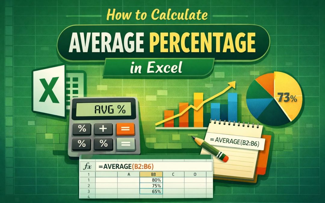
=AVERAGE(numbers)
How It Works
This formula tells Excel to add all the selected numbers and divide the total by the count of those numbers. You don’t have to do any division yourself—Excel does everything in one step.
Where to Use It
You can use the AVERAGE formula to calculate:
- Average marks of students
- Average monthly expenses
- Average scores in experiments
Example:
If the numbers are 10, 20, and 30, Excel calculates the average as 20.
How to Calculate Average in Excel (Step-by-Step)
Let’s look at how to calculate the average in Excel step by step.
Step 1: Enter the numbers in Excel cells (for example, marks in cells B1 to B5).
Step 2: Click on the cell where you want the average result.
Step 3: Type =AVERAGE(
Step 4: Select the range of cells (for example, B1:B5).
Step 5: Close the bracket and press Enter.
Example:
If marks are entered from B1 to B5, type:
=AVERAGE(B1:B5)
Excel will instantly display the average marks. Students can also type the cell references manually instead of selecting them with the mouse.
Different Ways to Calculate Average
Using the AVERAGE Function
This is the most common and easiest method. It works best for simple data sets like marks, prices, or scores.
Using the AutoSum Dropdown
Excel also provides an AutoSum option.
- Click on AutoSum (∑)
- Choose Average
- Highlight the numbers and press Enter
This method is very useful for beginners who are just learning Excel.
Calculating Average Manually in Excel
You can also calculate the average manually using a formula like:
=(B1+B2+B3+B4)/4
This method helps students understand the concept of average clearly, though it is not practical for large data.
AVERAGEIF (Conditional Average)
The AVERAGEIF function is used when you want to calculate the average of selected values only.
Example:
=AVERAGEIF(A1:A5, “>50”)
This formula calculates the average of only those numbers that are greater than 50.
Solved Examples
Example 1: Average Marks
Marks scored: 78, 85, 92
Formula used:
=AVERAGE(A1:A3)
Result: 85
Example 2: Average Expenses
Enter monthly expenses in a column and apply the AVERAGE formula to find the average monthly spending.
Example 3: Using AVERAGEIF
To find the average of marks above 60, use the AVERAGEIF function with the required condition.Common Mistakes Students Make
Students often make a few simple mistakes while calculating averages in Excel:
- Selecting blank cells along with numbers
- Entering text in cells meant for numbers
- Forgetting brackets in the formula
- Using commas instead of colons in ranges (A1,A5 instead of A1:A5)
Correct Example:
Use =AVERAGE(A1:A5) instead of incorrect formats.
Practice Exercises
Try these simple exercises in Excel:
- Enter the numbers 12, 18, 24, and 30. Find their average.
- Use =AVERAGE(A1:A6) to calculate the average height of students.
- Try =AVERAGEIF(A1:A5,”<50″) using your own sample values.
FAQs
What is the easiest way to find an average in Excel?
Using the AVERAGE function or the AutoSum → Average option is the easiest.
Can Excel find the average of selected cells only?
Yes, you can select specific cells or use the AVERAGEIF function.
Why does Excel show an error while calculating average?
This usually happens due to text values, wrong ranges, or missing brackets in the formula.
by Bethany Institutions | Dec 11, 2025
If you’ve ever opened an Excel sheet and felt overwhelmed because the same name or email appears again and again, trust me — you’re not alone. It happens to all of us. Maybe someone copied a list twice, maybe you pasted something in a hurry, or maybe the file has been passed around too many times. Either way, duplicates can make your data messy, confusing, and honestly a bit annoying.
The good news? Getting rid of them is much easier than people think. Excel actually has a built-in tool that cleans duplicates in seconds — and once you know where it is, you’ll wonder why you didn’t use it earlier.
Let me walk you through it in the simplest way possible.
What are duplicates, really?
Duplicates are just repeated entries.
That’s it. Nothing fancy.
For example:
- The same phone number typed twice
- Two rows with identical details
- An email ID that somehow appears five times
Left as it is, this can mess with your reports and throw off totals. Cleaning them keeps your data neat and dependable.
First step: Select the data
Before Excel can help you, it needs to know what to check.
You can:
- Highlight a single column
- Select multiple columns
- Or simply press Ctrl + A if you want it to look at everything
If you’re not sure where the duplicates are, Ctrl + A is the safest bet.
Next: Use Excel’s Remove Duplicates button
This is where the magic happens.
Go to the Data tab on top, and you’ll see a button called Remove Duplicates.
Click it.
No formulas, no complicated steps — just one button.
Now tell Excel what to compare
A small box pops up, showing your column names. This is Excel asking:
“Okay, what should I check for duplicates?”
If you only care about unique email IDs, select just the Email column.
If you want entire rows checked (meaning all values must match), select all columns.
Quick tip:
Tick the My data has headers option so Excel doesn’t treat your headings as actual data.
Time for the results
Hit OK and Excel will instantly scan your selection and clean things up.
You’ll get a message like:
“10 duplicate values found and removed; 90 unique values remain.”
It’s short, clear, and honestly feels a bit satisfying.
If you want to keep your original list untouched
Sometimes you don’t want Excel to delete anything — you just want a clean copy.
For that, there’s the Advanced Filter:
- Go to Data → Advanced
- Choose Copy to another location
- Tick Unique records only
- Select where you want the clean list to appear
Excel will place only the unique values in a new spot, leaving your original data safe.
If you prefer formulas
Some people enjoy formulas more than buttons. If that’s you, here are two useful ones:
For Excel 365 & 2021
=UNIQUE(range)
This immediately gives you a list of unique values.
For older Excel
=IF(COUNTIF($A$1:A1, A1)=1, A1, “”)
This one helps you spot duplicates by checking how many times a value has already appeared.
A quick keyboard shortcut
There isn’t a single key for removing duplicates, but this is the fastest keyboard method:
Alt → A → M
Literally just press those keys one after another:
- Alt opens the ribbon
- A goes to the Data tab
- M opens Remove Duplicates
Super quick once you get used to it.
A few things I always keep in mind
- I always take a backup before removing duplicates — just in case.
- Sometimes duplicates don’t look like duplicates because of extra spaces.
- Conditional Formatting (Home → Duplicate Values) is a great way to see duplicates before deleting them.
- If I’m unsure, I use the Advanced Filter method so nothing gets deleted accidentally.