How to Remove Blank Rows in Excel

by Bethany Institutions | May 6, 2026

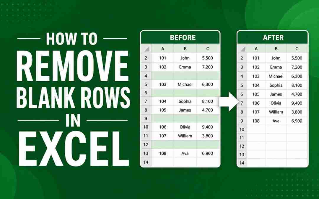
Blank rows in Excel are one of those little things that somehow cause big problems. You go to sort a list, and half your data ends up at the bottom. You write a quick formula, and it acts weird. Plus, honestly, it just looks sloppy if you’re sharing the file with anyone.

The good news? You can clean them up in a few seconds once you know the tricks. Here’s how.

The Fastest Way (Seriously, Learn This One)

If you forget everything else, remember this:

1. Select your data. Press Ctrl + A if you want to grab it all.
2. Hit Ctrl + G, click Special, then choose Blanks → OK.
3. Right-click any of the highlighted blank cells, pick Delete, then Entire row.
4. That’s it. They’re gone.

Takes about five seconds. Feels like magic the first time.

Why Bother Removing Blank Rows Anyway?

A couple of blank rows here and there doesn’t seem like a big deal. Until you try to sort. Or filter. Or use a pivot table. Then suddenly Excel acts like it’s never seen data before.

Blank rows also break things like basic math formulas. And if you’re sending the file to your boss or a client, those random empty lines just look unfinished. So yeah, worth cleaning up.

Method 1 – Go To Special (The One I Actually Use)

Steps:

• Select everything. (Ctrl + A twice if your data is in a nice block.)
• Ctrl + G → Special → Blanks.
• Right-click a highlighted cell → Delete → Entire row.

When to reach for this:
Pretty much anytime your data is clean and rectangular—sales reports, expense lists, customer emails. No extra columns, no filters, no fuss.

Method 2 – Filter Feature (Safer When You’re Unsure)

Steps:

• Click anywhere inside your data.
• Go to the Data tab → Filter (or just press Ctrl + Shift + L).
• Click the dropdown arrow on any column. Uncheck “Select All,” then check (Blanks).
• Select all the visible blank rows (click the first row number, hold Shift, click the last).
• Right-click → Delete row.
• Turn off the filter.

When to use this:
Big spreadsheets where you want to see what you’re deleting first. Or when blanks only exist in certain columns—this way you don’t accidentally delete rows that have data elsewhere.

Method 3 – Sort and Delete (Lazy but Effective)

Steps:

• Select your data range.
• Sort by any column (A to Z works fine).
• All the blank rows will move to the bottom automatically.
• Just select those bottom rows and delete them.

When to use this:
When you’re in a rush and don’t feel like remembering shortcuts. Warning though—this reorders your data. So if row order matters (like dates or sequences), skip this one.

Method 4 – Formula + Helper Column (For Messy Data)

Steps:

• Add a new column at the end. Call it something like “Empty?”
• In row 2, type: =COUNTA(A2:Z2)=0 (change the range to cover all your columns).
• Drag that formula all the way down.
• Filter or sort on that column for TRUE, then delete those rows.

When to use this:
You only want to delete rows that are completely empty. Or your data has weird stuff like spaces or formulas that return “” (those aren’t technically blank, but you still want them gone). This catches all of it.

Method 5 – Power Query (Fancy but Worth It)

Steps:

• Select your data → Data tab → From Table/Range.
• In the Power Query editor, click Remove Rows → Remove Blank Rows.
• Click Close & Load.

When to use this:
You clean the same report every week. Power Query remembers the steps, so next time you just hit refresh. Also handles huge datasets that make regular Excel freeze up.

Mistakes People Make (Me Included)

• Deleting cells instead of rows – This leaves blank cells scattered around. Always pick “Delete entire row.”
• Not selecting everything first – If you only highlight one column, Excel deletes rows based on that column alone. You might lose good data in other columns.
• Forgetting about invisible blanks – Some cells look empty but have spaces, line breaks, or formulas returning “”. The methods above won’t catch those unless you clean them first. Try =TRIM(CLEAN(A1)) if that’s happening.

A Few Tips to Make This Faster

• Ctrl + Shift + L turns filters on and off instantly. Use it.
• Turn your data into a Table (Ctrl + T). Tables remember filter settings and auto-expand ranges.
• Quick check for hidden junk: Select your data, hit Ctrl + H, leave Find what blank, replace with “CHECK”. If anything changes, you have invisible characters.

So Which One Should You Actually Use?

• Go To Special – everyday stuff. Fast and easy.
• Filter – big files or when you want to be careful.
• Sort – speed is king and order doesn’t matter.
• Helper formula – only delete fully empty rows.
• Power Query – same report over and over again.

Honestly? Most of the time I just use Go To Special. It’s short, it works, and I don’t have to think.

FAQs

How do I delete blank rows quickly?
Ctrl + G → Special → Blanks → right-click → Delete row. Seriously, try it once and you’ll remember forever.

Can I remove blank rows without messing up my other data?
Yes, as long as you select everything first. If you only select part of the sheet, you’ll shift things out of alignment.

What’s the absolute fastest method in Excel?
Go To Special. No extra columns, no sorting, no formulas. Just a few clicks.

How to remove blank rows in huge datasets (like 100k+ rows)?
Use Power Query or the filter method. Sorting gets slow on that much data. Power Query handles it like a champ.

How to Create a Pivot Table in Excel

by Bethany Institutions | Apr 27, 2026

Let’s Be Real for a Second

You’ve got an Excel sheet open. It’s huge. You’re scrolling. Your eyes are glazing over. And somewhere in the back of your mind, you’re thinking, “There’s no way I’m going through all this manually.”

I’ve been there. More times than I’d like to admit.

The first time someone showed me a pivot table, I literally said, “Wait… that’s it?” It felt like cheating. A few clicks, and suddenly all that messy data turned into something I could actually make sense of.

If you’ve never used one before, don’t worry. I’ll walk you through it like we’re sitting next to each other.

So… What Even Is a Pivot Table?

Honestly? It’s just a tool that helps you stop staring at rows of numbers and start understanding them.

With a pivot table, you can:

• Add stuff up
• Find averages
• Group things together
• Spot patterns you’d never notice otherwise

And the best part? No formulas. No headaches. You just drag and drop, and Excel does the rest.

Want to see total sales by month? Done.
Break down expenses by category? Easy.
Analyse student marks by subject? Takes seconds.

Oh, and it’s called a “pivot” table because you can literally pivot—turn the data around—whenever you want to look at it differently.

One Thing Before You Start (Seriously, Do This)

I learned this the hard way, so let me save you the trouble.

Before you create a pivot table, take a quick look at your data:

• Make sure every column has a heading (no blanks—Excel gets confused)
• No empty rows hiding in the middle
• Each column has one type of data (don’t mix numbers and text)
• No merged cells (they cause chaos)

Also, check that your numbers are actually numbers and your dates are dates. Excel can be picky.

Here’s a trick I always use:
Hit Ctrl + T to turn your data into a table. It sounds small, but it makes everything smoother—especially when you add more data later.

How to create a pivot table in Excel step by step

Ready? This is easier than you think.

Step 1: Click Anywhere in Your Data

You don’t need to highlight everything. Just click inside the dataset somewhere.

Step 2: Go to Insert → PivotTable

Up at the top, click Insert, then PivotTable.

Step 3: Pick a Spot

A little box pops up. Excel already knows your data range. Just choose New Worksheet (it keeps things tidy) and hit OK.

Step 4: Don’t Freak Out at the Blank Screen

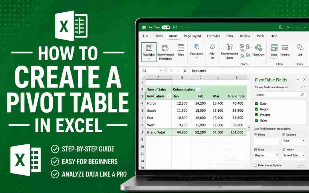
You’ll see a blank grid on the left and a panel on the right. That panel is where all the magic happens.

Step 5: Drag and Drop (This Is the Fun Part)

You’ll see four boxes:

• Rows → things you want listed (like product names or regions)
• Columns → how you want to compare (like months or years)
• Values → the numbers you want to calculate (like sales or counts)
• Filters → optional filters if you want to narrow things down

Just drag fields into those boxes and watch Excel build your report instantly. It feels almost too easy.

Step 6: You’re Done

Seriously. That’s it.

Now go ahead—move things around, remove stuff, try different combinations. You won’t break anything. I promise.

How to Make It Actually Useful

A basic pivot table is great. But a few small tweaks can make it feel like magic.

Change What You’re Calculating

By default, Excel sums things up. But what if you want an average instead?

Right-click any number → Value Field Settings → pick Average, Count, or whatever you need.

Filter Without Messing Around

Want to see just one region or one product? Use the dropdowns on the table.

Or go a step further…

Use Slicers (They’re Awesome)

Go to PivotTable Analyse → Insert Slicer. You’ll get clickable buttons that filter your data. It’s clean, visual, and honestly makes you look like an Excel pro.

Excel slicers tutorial

Sort So You Actually See What Matters

Click the dropdown on your row labels and sort from largest to smallest. That way, you spot the big stuff first.

Refresh When Your Data Changes

This one trips everyone up at first.

If you update your original data, your pivot table doesn’t update automatically. Just right-click it and hit Refresh. That’s it.

Want a Chart? Add a Pivot Chart

Sometimes numbers alone don’t tell the full story.

Click your pivot table → PivotTable Analyse → PivotChart → pick a chart type.

Done. And the best part? The chart updates whenever your pivot table changes. No extra work.

Mistakes I’ve Made (So You Don’t Have To)

Let me save you some frustration:

• Blank headers → Excel throws a fit. Just don’t.
• Numbers stored as text → your calculations won’t work. Check formatting.
• Forgetting to refresh → you’ll wonder why your numbers look old. Refresh!
• New rows not included → if you add data, your pivot table won’t see it unless you converted to a table first (Ctrl + T fixes this).

A Few Things I Wish Someone Told Me Earlier

Once you start using pivot tables, these little things make a big difference:

• Use slicers for filtering. They’re not just useful—they’re actually nice to look at.
• Group dates by month or year with a right-click. So handy.
• Duplicate your pivot table to try different views without messing up your original one.
• Use conditional formatting to highlight big numbers automatically.
• Keep your original data clean. Future you will be grateful.

Alright, Here’s the Truth

If you’ve followed along, you’ve already done the hardest part—getting started.

Pivot tables look intimidating. I get it. But once you try them, you’ll realize they’re actually one of the easiest tools in Excel. And more importantly, they save you so much time.

Next time you’re staring at a huge dataset, don’t torture yourself trying to do it manually.

Just create a pivot table.

You’ll have your answer in seconds. And you’ll wonder why you didn’t try it sooner.

FAQs

What is a pivot table?
It’s a tool that helps you summarize and understand big sets of data without using formulas.

How do I make one as a beginner?
Click your data → Insert → PivotTable → drag fields into Rows, Columns, and Values. That’s literally it.

Does it update when my data changes?
Only if you right-click and hit Refresh. Easy.

What’s the difference between a pivot table and a normal table?
A normal table just shows your data. A pivot table actually helps you make sense of it.

Can I make a chart from it?
Yes, and it’s called a PivotChart. It updates automatically when your pivot table changes

How to Freeze Multiple Columns in Excel

by Bethany Institutions | Mar 2, 2026

If you’ve ever worked on a large Excel sheet, you know the struggle. You scroll to the right to check some data, and suddenly the names, IDs, or categories on the left vanish. Now you’re guessing which row belongs to what—and that’s how mistakes happen.

Freezing columns in Excel solves this problem neatly. It lets you keep important columns visible while you scroll through the rest of the sheet. In this guide, I’ll show you how to freeze multiple columns in Excel, when it makes sense to use this feature, and a few common mistakes to watch out for.

What Does Freezing Columns Mean in Excel?

Freezing columns in Excel simply means locking certain columns in place so they stay visible when you scroll horizontally. The data doesn’t change—only how it appears on your screen.

This is different from hiding columns. When you hide a column, it disappears completely. Freezing keeps the column visible at all times, which is far more useful when you need constant reference.

You’ll often see frozen columns used in:

• Student records and attendance sheets
• Sales and finance reports
• Large tracking or comparison sheets 

Basically, anytime the first few columns matter, freezing is a smart move.

When Should You Freeze Multiple Columns in Excel?

Freezing multiple columns is especially helpful when:

• You’re working with wide spreadsheets that stretch across many columns
• Important reference details like names, roll numbers, or product IDs need to stay visible
• You’re comparing data across several columns
• You’re doing data entry or verification and want to avoid mix-ups 

If you’re constantly scrolling left just to remind yourself what a row refers to, it’s time to freeze those columns.

How to Freeze Multiple Columns in Excel (Step-by-Step)

Step 1 – Select the Right Column

This is the part most people get wrong the first time.

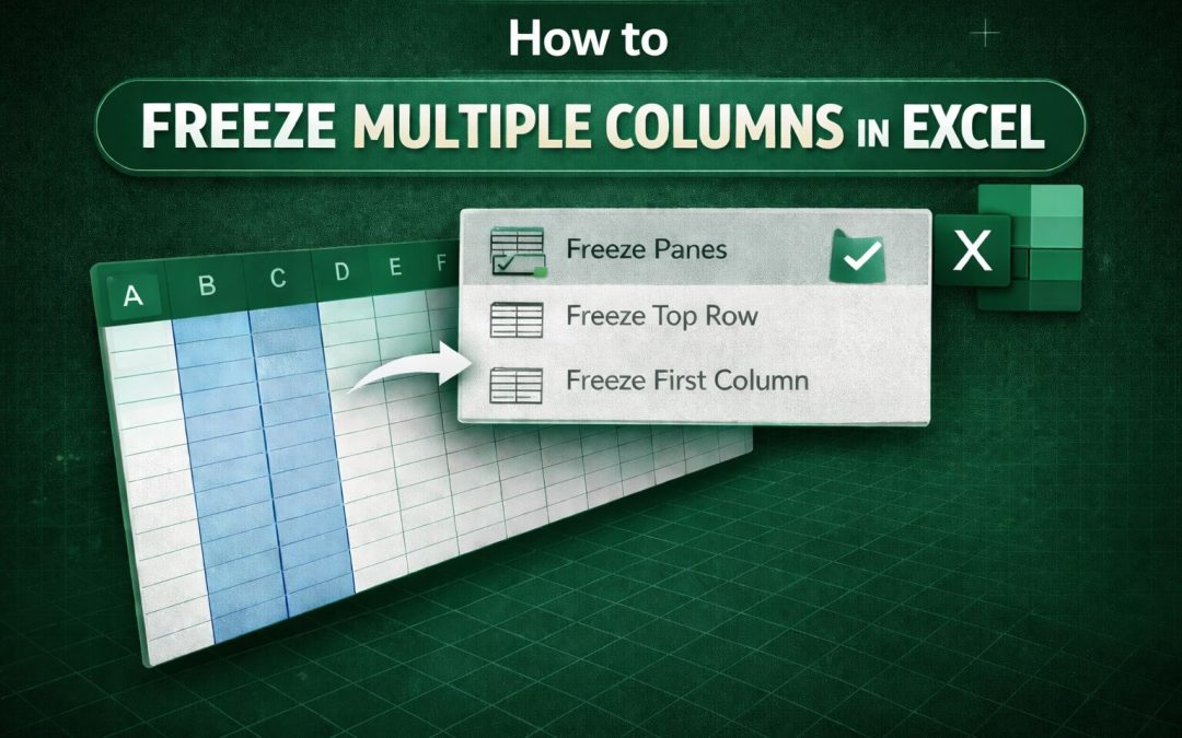
Excel freezes everything to the left of the column you select.

Example:
If you want to freeze Column A and Column B, click on Column C.

Step 2 – Open the Freeze Panes Option

• Go to the View tab at the top
• Click on Freeze Panes 

Step 3 – Click Freeze Panes

• Select Freeze Panes from the dropdown
• Excel will immediately freeze the selected columns 

You’ll see a thin grey line showing where the freeze starts.

How to Freeze Both Rows and Multiple Columns Together

Sometimes you want the best of both worlds—frozen headers at the top and frozen columns on the side.

Here’s how:

• Click the cell that is below the rows and to the right of the columns you want to freeze
• Go to View → Freeze Panes → Freeze Panes 

This works beautifully for large reports where headings and key reference columns need to stay visible at all times.

How to Unfreeze Columns in Excel

If you want to remove the freeze:

• Go to the View tab
• Click Freeze Panes
• Choose Unfreeze Panes 

Your sheet will return to normal scrolling instantly.

Common Mistakes to Avoid

• Selecting the wrong column before clicking Freeze Panes
• Trying to freeze columns after scrolling far across the sheet
• Mixing up Freeze Panes with the Split option
• Forgetting to unfreeze columns before sharing the file with others

These are small mistakes, but they can cause a lot of confusion.

Pro Tips for Smoother Excel Work

• Freeze only the most important columns—too many can feel cluttered
• Combine frozen rows and columns for large datasets
• Use freezing in dashboards, trackers, and monthly reports

Once you get used to it, freezing becomes second nature.

Conclusion

Freezing multiple columns in Excel is a simple feature, but it makes a huge difference when working with large spreadsheets. It keeps important information visible, reduces scrolling back and forth, and helps prevent errors. Whether you’re handling student data, financial reports, or tracking sheets, freezing columns can save time and make your work much easier. Best of all, it’s quick to set up and just as easy to remove.

FAQs

How many columns can I freeze in Excel?
You can freeze as many adjacent columns as you want.

Can I freeze columns and rows at the same time?
Yes, just select the correct cell and use Freeze Panes.

Why is the Freeze Panes option greyed out?
This usually happens if you’re editing a cell or working in a protected sheet.

How do I freeze the first two columns quickly?
Select Column C, then go to View → Freeze Panes → Freeze Panes.

What’s the difference between Freeze Panes and Split?
Freeze Panes locks parts of the sheet, while Split only divides the screen for viewing.

Does freezing affect formulas or data?
No. It only changes how the sheet looks on your screen.

How to Merge & Centre Cells in Excel

by Bethany Institutions | Feb 20, 2026

If you’ve ever looked at an Excel sheet and thought, “This looks messy”, formatting is usually the problem—not the data. Simple things like aligning text or merging cells can make a huge difference, especially when you’re working on reports, headers, tables, or dashboards. One of the most commonly used tools for this is Merge & Centre. Let me show you how it works, when to use it, and when it’s better to avoid it.

What Does Merge & Centre Mean in Excel?

Merge & Centre does exactly what the name suggests, but it helps to break it down.

Merging cells

When you merge cells, you’re combining two or more neighbouring cells into one larger cell. For example, merging A1, B1, and C1 turns them into a single wide cell.

Centring text

Once the cells are merged, Excel automatically places the text in the centre of that new cell. This makes headings stand out and keeps things visually balanced.

When is it usually used?

Most people use Merge & Centre for:

• Titles at the top of reports

• Headings above tables

• Section labels

• Dashboard headings

It’s mainly a presentation tool, not a data-management one.

How to Merge & Centre Cells in Excel

There are a couple of easy ways to do this. The first one is what most users start with.

Method 1 – Using the Merge & Centre Button

1. Select the cells you want to merge

2. Go to the Home tab

3. Click Merge & Centre

That’s it. The cells merge, and the text moves neatly into the centre.

Method 2 – Using the Merge Options Dropdown

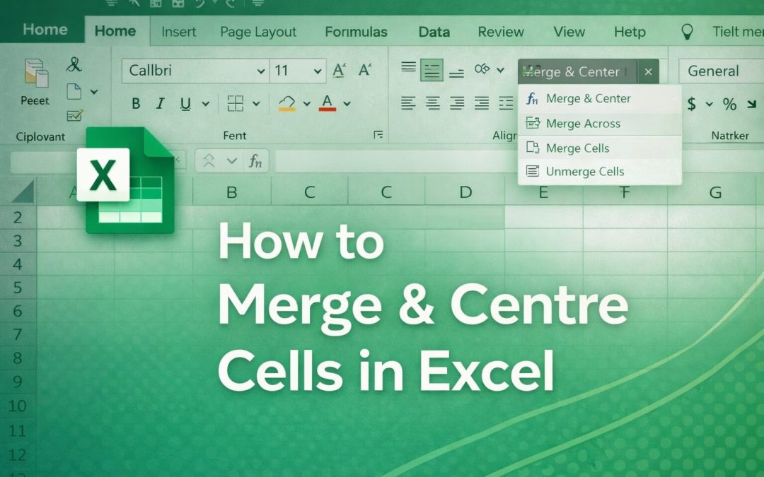
Next to the Merge & Centre button, you’ll notice a small arrow. Clicking this opens more options:

• Merge & Centre

• Merge Across

• Merge Cells

• Unmerge Cells

Each option is useful in different situations.

Understanding the Different Merge Options

Merge & Centre

This is the most popular option. It merges the selected cells and centres the text automatically. Best for titles and headers.

Merge Cells

This merges cells but doesn’t change the text alignment. If you want the text left-aligned or right-aligned, this option gives you more control.

Merge Across

This merges cells row by row instead of merging everything into one big cell. It’s handy when working with structured layouts.

Unmerge Cells

This splits a merged cell back into individual cells. Just remember—only the top-left cell keeps the data.

How to Merge Cells Without Centring Text

There are times when centring text doesn’t look right, especially in tables.

To merge without centring:

1. Select the cells

2. Click the Merge & Centre dropdown

3. Choose Merge Cells

This keeps your layout clean while letting you control text alignment manually.

How to Unmerge Cells in Excel

Unmerging is just as simple as merging.

1. Select the merged cell

2. Go to Home → Merge & Centre dropdown

3. Click Unmerge Cells

What happens to the data?

Only the content in the top-left cell stays. Everything else is cleared, so it’s always smart to double-check before unmerging.

When Should You Use Merge & Centre?

Merge & Centre works best when it’s used in the right places.

Good examples include:

• Report titles

• Section headers

• Dashboard headings

• Excel sheets meant for printing

These areas benefit from better spacing and visual clarity.

Common Mistakes to Avoid

This is where many people run into trouble.

Losing data while merging

When cells are merged, Excel keeps only the top-left value. Any other data is removed without warning.

Using merged cells inside data tables

Merged cells can interfere with:

• Sorting

• Filtering

• Pivot tables

If your data needs to be analysed, avoid merging.

Overusing merged cells

Too many merged cells make a sheet harder to edit and maintain later.

Formula problems

Merged cells can cause reference issues in formulas, especially in larger sheets.

A Few Simple Formatting Tips

If you want your Excel sheets to look good and work smoothly:

• Use Centre Across Selection instead of merging when possible

• Avoid merging cells in datasets used for calculations

• Reserve merged cells mainly for headings and titles

These small habits save a lot of frustration later.

Conclusion

Merge & Centre is a great tool when your goal is better presentation and readability. It helps headings stand out and makes reports look more polished. That said, it’s best used carefully and mostly outside of working data tables. Always check your data before merging, and remember—good formatting should make your work easier, not harder.

FAQs

What happens to data when I merge cells?
Only the top-left value remains. All other data is deleted.

Can I merge cells without centering text?
Yes. Use the Merge Cells option instead of Merge & Centre .

Why is Merge & Centre sometimes disabled?
This can happen if the sheet is protected, you’re editing a cell, or you’re working inside a table.

Does Merge & Centre affect formulas?
Yes. Merged cells can cause formula and reference issues.

How do I unmerge cells without losing data?
Excel doesn’t restore deleted values, so always copy data before unmerging.

Is Merge & Centre good for data tables?
No. It’s best avoided in tables used for sorting, filtering, or analysis.

How to Insert a New Row or Column in Excel

by Bethany Institutions | Feb 19, 2026

Introduction

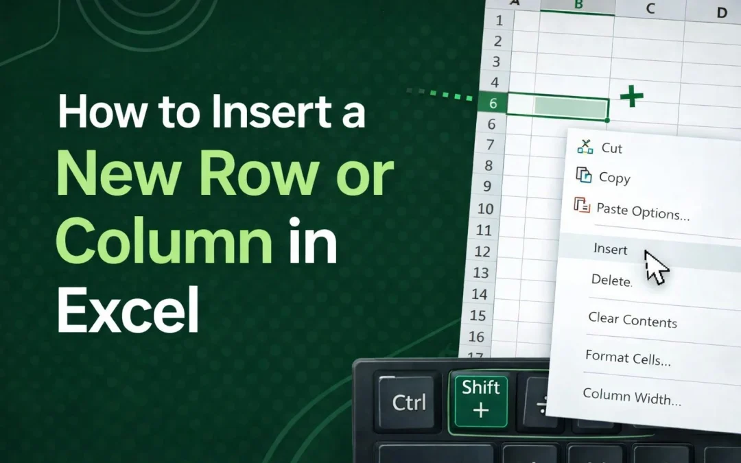
Let’s be honest—most of us open Excel almost on autopilot. It could be to update marks, track expenses, prepare a report, or organise data for work or college. And while Excel can do a lot of advanced things, it’s the basic skills that really make daily work easier. One of those basics is knowing how to insert rows and columns properly. Doing this the right way helps you keep your data neat, avoid overwriting important information, and save time. In this article, I’ll walk you through simple methods, keyboard shortcuts, and a few common mistakes to watch out for.

What Does Inserting a Row or Column Mean in Excel?

Before getting into the steps, it’s useful to understand what Excel actually does when you insert something.

When you insert a row, Excel creates a new blank row and shifts all the existing data below it downward. Nothing is deleted—your data simply moves to make space.

When you insert a column, Excel adds a new column and pushes the existing columns to the right.

This is much safer than typing over existing cells. Instead of risking data loss, inserting rows or columns keeps everything organised and intact.

How to Insert a New Row in Excel

Method 1 – Using Right Click

This is the easiest and most commonly used method.

1. Click on the row number where you want to add a new row.
2. Right-click on that row number.
3. Select Insert.

Excel will add a new row just above the selected row.

Method 2 – Using Keyboard Shortcut

If you use Excel often, shortcuts can save you a surprising amount of time.

Shortcut: Ctrl + Shift + +

Steps:

1. Select the entire row by clicking its row number.
2. Press Ctrl + Shift + +.

This shortcut is especially helpful when you need to insert rows quickly without using the mouse.

Method 3 – Using the Excel Ribbon

If you prefer menu options, this method works well.

1. Select the row.
2. Go to the Home tab.
3. Click Insert in the Cells section.
4. Choose Insert Sheet Rows.

How to Insert a New Column in Excel

Method 1 – Using Right Click

1. Click on the column letter where you want the new column.
2. Right-click on the column header.
3. Click Insert.

The new column will appear to the left of the selected column.

Method 2 – Using Keyboard Shortcut

The shortcut for inserting a column is exactly the same as inserting a row.

Shortcut: Ctrl + Shift + +

Steps:

1. Select the full column by clicking its letter.
2. Press Ctrl + Shift + +.

This is one of the most searched Excel shortcuts—and once you get used to it, you’ll use it all the time.

Method 3 – Using the Excel Ribbon

1. Select the column.
2. Go to Home → Insert.
3. Click Insert Sheet Columns.

How to Insert Multiple Rows or Columns in Excel

There are times when inserting just one row or column isn’t enough.

Inserting Multiple Rows

1. Select the same number of rows as you want to insert.
2. Right-click and choose Insert, or press Ctrl + Shift + +.

Excel will insert the new rows above your selection.

Inserting Multiple Columns

1. Select multiple columns by dragging across the column letters.
2. Right-click and choose Insert.

This is especially useful when working with large datasets or adding monthly or yearly data.

How to Insert Rows or Columns in Excel Tables

If your data is formatted as an Excel Table, things become even easier.

• Tables automatically expand when you insert new rows or columns.
• Formatting stays consistent.
• Formulas are copied automatically.

To insert a row in a table:

• Click anywhere inside the table.
• Right-click → Insert → Table Rows Above or Below.

For large or important datasets, tables are a safer option because Excel handles most of the structure for you.

Common Mistakes to Avoid

Even though inserting rows and columns is simple, a few mistakes can cause confusion later.

• Not selecting the entire row or column before inserting.
• Trying to insert rows within merged cells.
• Forgetting to check formulas after inserting new data.
• Inserting rows in filtered sheets without checking how Excel applies the change.

Taking a moment to check these things can save a lot of trouble later.

Pro Tips for Faster Excel Work

If you want to work more confidently in Excel, these small tips help:

• Get comfortable with keyboard shortcuts—they really do speed things up.
• Convert your data into tables before making major changes.
• Save your file before inserting multiple rows or columns.

These habits make Excel feel far less stressful.

Conclusion

Inserting rows and columns may seem like a small thing, but it’s a skill you’ll use constantly in Excel. Whether you prefer right-clicking, using shortcuts, or working through the ribbon, Excel gives you plenty of options. Once you start using shortcuts regularly, your work becomes faster and smoother. Just remember to keep an eye on formulas and formatting, especially when dealing with larger sheets.

FAQs

How do I insert a row using a shortcut?
Select the row and press Ctrl + Shift + +.

Does inserting a row affect formulas?
Most of the time, Excel updates formulas automatically, but it’s always wise to double-check.

How do I insert a row between two rows?
Select the row below, right-click, and choose Insert.

Can I insert rows in filtered data?
Yes, but be careful—Excel may insert rows only into visible data.

How do I insert multiple rows at once?
Select multiple rows first, then insert them together.

Why is the insert option sometimes disabled?
This usually happens because of merged cells or protected worksheets.